
Filter in Google Sheets: Explained
In this article, you will learn what a filter is and how to use them in Google Sheets.
A filter is beneficial when you want to look at relevant items or have a sorted list of items in a large volume of data because the function has various options to re-order items and show things that meet a criterion. If you want to save and share the filter you create, you should use Filter Views instead.
How to use Filter in Google Sheets
- Prepare a data set ideally with table headers and select its entire range.
- Go to the “Data” tab → “Create a filter”.
- Navigate to the column header based on which you want to sort.
- Click the icon shaped like an inverted triangle next to the header.
- Define how to sort the column in the menu and click the “OK” button.

When you click the reverse triangle icon, you will see the filtering menu, as shown below.

Sort A → Z: You can reorder items in alphabetical order
Sort Z → A: Things are rearranged in reverse alphabetical order
Sort by color (Fill color): The values are sorted based on cell colors - conditional formatting colors work for this filter, but alternating colors do not.
Sort by color (Text color): You can organize data based on text colors
Filter by condition: The items are selected by one of the default conditions relevant to text, date, and number (e.g., “Text contains”, “Date is”, and “Greater than”) or your own rule defined under “Custom formula is”.
Filter by values: The values are shown when the boxes next to them are checked and hidden if they are unchecked.
Lastly, look at the example below. Assume you have the following records. You want to focus on people from the “North” country.

- Go to the reverse triangle icon next to “Country”.
- Navigate to “Filter by values”.
- Uncheck the boxes next to countries except for “North”.
- Click the “OK” button on the bottom right.
Note: Look at “Select all” and “Clear” beneath “Filter by values”. If you click “Select all”, all boxes are checked. On the other hand, if you click “Clear”, all checkboxes are unchecked. They are helpful when you want to check or uncheck multiple items.

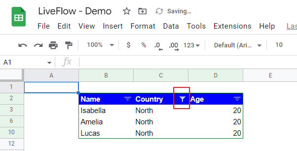
The following screenshot shows the filtered result. As you can see, the inverted triangle has turned into a funnel icon, which means the column is filtered.
How can I delete a filter?
If you want to delete the filter, navigate to the “Data” tab → “Remove filter”.
Can I save a filter as Filter View?
Yes, you can. Navigate to “Click Data” → “Filter views” → “Save as filter view”. Check this article to learn Filter View and how to use it.
How does a filter affect other collaborators?
When you create a filter, collaborators who have access to a worksheet can see the filter. Also, collaborators who have permission to edit the spreadsheet can change the filter setting.